Comment construire un graphe PERT minimal/How to construct a minimal PERT graph ∗†
Translated: April 30, 2019
∗Reçu février 1979./Received February 1979.
†Lien vers l’article original/Link to original paper
‡ Université de Lille-I, Villeneuve-d’Ascq, France./Université de Lille-I, Villeneuve-d’Ascq, France.
Abstract
| Nous donnons un algorithme permettant, pour un problème d’ordonnancement donné, de construire le graphe PERT ayant un nombre minimal de sommets. Cet article contient la preuve de la validité de l’algorithme, un example et des résultats numériques. Mote clés: ordonnancement, graphe PERT minimal, algorithme de construction de graphes. | We give an algorithm for constructing, for a given project scheduling problem, the PERT graph having the smallest number of vertices. This paper contains a proof of the validity of the algorithm, an example and numerical results. Keywords: scheduling, minimal PERT graph, graph construction algorithm. |
Introduction/Introduction
| Le problèmes d’ordonnancement sont définis par la donnée d’un certain nombre d’opérations (les tâches) et des contraintes de succession entre ces tâches (la tâche ne peut commencer qu’après que la tâche soit terminée), ainsi que les durées de chacune de ces tâches. | Scheduling problems are defined by data consisting of a certain number of operations (tasks) and constraints on the ordering of these tasks (task can not start until task has finished) as well as the duration of each of these tasks. |
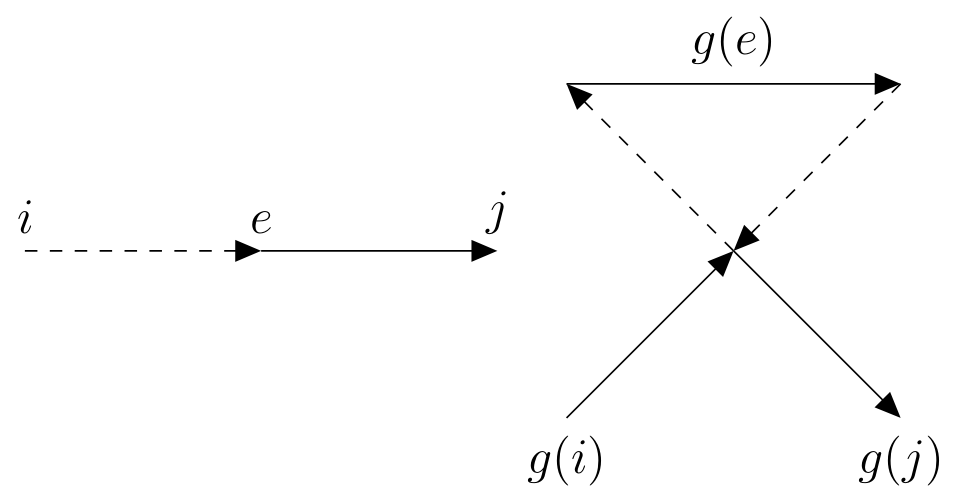
| Définir un ordonnancement consiste à attribuer à chacune des tâches une date d’exécution de manière à ce que l’ensemble des tâches soit terminé au plus tôt. Une des méthodes pour résoudre ce problème est la méthode PERT [1, 2]. Le premier pas de cette méthode consiste à construire un graphe (graphe PERT ou américain) dont les arcs représentent les tâches et où les relations de succession entre les tâches sont traduites ainsi : est successeur de si et seulement si il existe dans le graphe un chemin dont le premier arc est et le dernier . La construction n’est en général possible que si l’on introduit de nouvelles tâches, dites virtuelles, de durée nulle. | Creating a schedule consists of assigning each task a date of execution so that all tasks are completed as early as possible. One of the methods for solving this problem is the PERT method [1, 2]. The first step of this method is to construction a graph (PERT or American graph) whose arcs represent the tasks and where the succession relations between tasks is translated as follows: is the successor of if and only if there exists a path in the graph whose first arc is and last one is . The construction is usually possible only if we introduce new tasks, called virtuals, that are of zero duration. |
|
Kelley [3] note qu’il est avantageux pour réduire la longueur des calculs suivants de construire un graphe PERT ayant le nombre minimal possible de sommets. Le problème ainsi posé par Kelley a été abordé avec plus ou moins de succès par un certain nombre d’auteurs: Hayes [4] donne un ensemble de recettes pour construire un graphe PERT. Sa méthode ne produit pas, en général, le graphe minimal. Dimsdale [5] propose un algorithme de construction du graphe PERT minimal. Fisher, Liebman, Nemhauser [6] montrent que l’algorithme de Dimsdale est faux; ils en donnent un nouveau qui est exact; leur article ne contient pas de preuve mathématique conformément au style du journal (C.A.C.M.). Cantor et Dimsdale [7] donnent, avec démonstration, un algorithme exact. Leur méthode qui s’applique à un problème qui englobe les problèmes d’ordonnancement, gagne en généralité mais donne lieu, pour notre cas particulier, à des calculs inutilement longs. Syslo [8] cherche à minimiser le nombre des arcs virtuels ce qui est un autre problème. Dans le présent article notre contribution est la suivante : comme dans [6] nous ne considérons que le problème d’ordonnancement (ceci implique en particulier que les relations de succession entre tâches réelles ne peuvent pas former de circuit). Nous reprenons certaines notions des articles ci-dessus ou nous en définissons d’autres qui sont voisines. Nous démontrons certaines propriétés (notamment le théorème 1) qui ont échappé aux auteurs précédents et qui permettent finalement de donner un algorithme de construction du graphe PERT minimal réduisant le nombre des calculs. |
Kelley [3] notes that it is advantageous to reduce the length of the following calculations by constructing a PERT graph that has the minimal possible number of vertices. The problem thus posed by Kelley has been addressed with varying degrees of success by a certain number of authors: Hayes [4] gives a set of recipes for constructing a PERT graph. His method does not produce, in general, the minimal graph. Dimsdale [5] proposes an algorithm for the construction of the minimal PERT graph. Fisher, Liebman, Nemhauser [6] show that Dimsdale’s algorithm is false; they give a new one that is exact; their article does not contain a mathematical proof that complies with the journal style (C.A.C.M). Cantor and Dimsdale [7] give, with demonstration, an exact algorithm. Their method, which applies to a problem that includes scheduling problems, works in general, but gives rise to unnecessarily long calculations for our particular case. Syslo [8] tries to minimise the number of virtual arcs which is another problem. In this article our contribution is as follows: as in [6] we only consider the scheduling problem (this implies in particular that the successive relations between real tasks can not form a circuit). We take up some notions from the above articles or we define other related ones. We demonstrate certain properties (in particular Theorem 1) that have escaped the previous authors and finally allow us to give an algorithm for the construction of the minimal PERT graph that reduces the number of calculations. |
1 Notations et définitions/Notation and definitions
2 Construction/Construction
2.1 Graphe : construction et propriétés/ graph: construction and properties
2.2 Graphe : construction et propriétés/ graph: construction and properties
| Dans le graphe on pose: et On vérifie aisément que les deux relations et sont des relations d’équivalence; soient les classes correspondantes sur et . On appelle contraction de type 1 l’opération qui consiste dans à contracter, en un sommet unique, tous les sommets d’une même classe.
| In the graph , we let and
It is easy to verify that the two relations and are equivalence relations; are the corresponding classes on and . We call type 1 contraction the operation that contracts all vertices of of the same class to a single vertex.
|
Construction du graphe / Construction of graph
Définition d’un bon arc de /Definition of a good arc of
|
Un arc est un bon arc de : On appelle contraction de type 2 l’opération qui, dans , consiste à contracter, en un sommet unique, le sommet origine et le sommet extrêmité d’un bon arc. Remarque 2.2.2 On vérifie aisément qu’une contraction de type 2 ne supprime aucune relation de succession entre arcs réels qui existait initialement. Remarque 2.2.3 On vérifie aisément que la définition d’un bon arc est équivalente à la suivante:Théorème 1 Les bons arcs de n’ont deux à deux aucun sommet commun.
|
An arc is an good arc of : We call contraction de type 2 an operation where, in , consists of contraction, in one unique vertex, the origin vertex and destination vertex of a good arc. Remark 2.2.2 It can be easily verfied that a type 2 contraction does not remove any succession relation between real arcs that initially exist. Remark 2.2.3 It can be easily verified that the defiintion of a good arc is equivalent to the following:Theorem 1 The good arcs of do not have two common pairs of vertices.
|
2.3 Graphe : construction et propriétés/ graph : construction and properties
Construction du graphe /Construction of graph
|
Dans le graphe
on effectue toutes les contractions possibles
de type 2. Soit
le graphe obtenu. Dans le but de simplifier les notations:
|
In the graph
we perform all the possible type 2
contractions. is
the obtained graph. In order to simplify the notation:
|
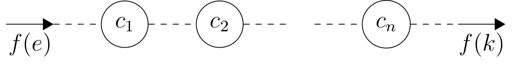
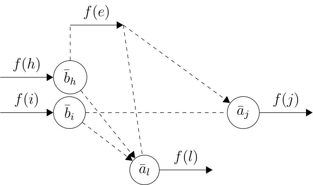
| Les sommets intermédiaires proviennent de la contraction des bons arcs de (fig. 3). | The intermediate vertices from the contraction of the good arcs of (fig. 3). |
|
Comme est un bon arc, et implique . Comme est un bon arc, et d’après la remarque 2.2.3, et implique . On démontre ainsi de proche en proche que jusqu’à , et finalement . Montrons que, parmi les graphes arcs-duaux du graphe a le nombre minimal de sommets. Ce sera une conséquence du théorème suivant. Théorème 2 Soit le graphe arc-dual de par l’application construit précédemment et soit un autre graphe arc-dual de par l’application . Alors il existe et une application surjective de sur telle que :
Démonstration :
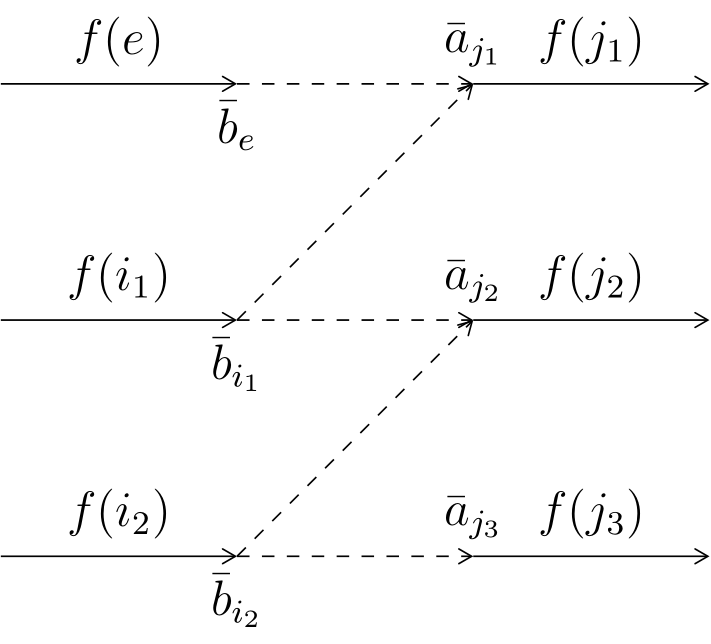
Construction de . Soit , avec et on pose et . Montrons que est bien définie. Soit , avec et ; posons et (a) Montrons que si dans alors dans . Il faut donc montrer que dans . Soit . Comme est arc-dual de , on a . Comme et ont la même origine, on a , d’où dans . Si on avait , il existerait un sommet de tel que et (fig. 4). |
Since is a good arc, and implies . Since is a good arc, and according to remark 2.2.3, and implies . We thus prove step by step that up to , and finally . We show that, among the dual-arc graphs of , has the minimal number of vertices. This will be a consequence of the following theorem. Theorem 2 Let be the dual-arc graph of by the mapping previously constructed and let be another dual-arc graph of by mapping . Then there exists and and a surjective map of on such that:
Demonstration :
Construction of . Let , with and we pose and . Let us
show that
is well-defined. Let , with and ; let us pose and (a) Let us show that if in then in . We must therefore show that in . Let . Since is a dual-arc of , we have . Since and have the same origin, we have , hence in . If we had , there would exist a vertex of such that and (fig. 4). |
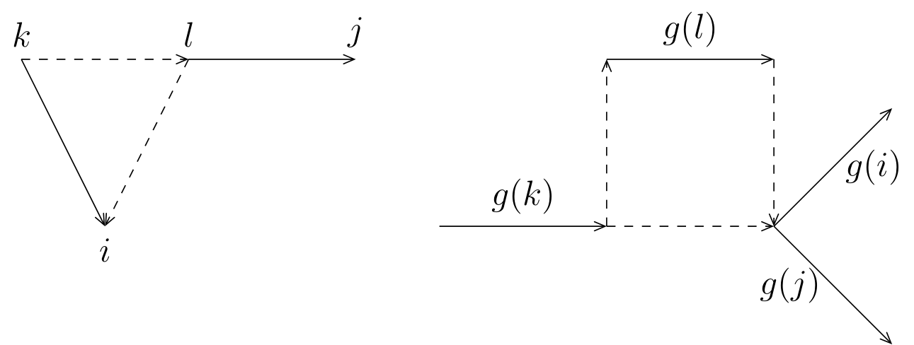
| Comme ci-dessus, du fait que et que et ont la même origine, on a , et . L’arc serait alors redondant dans , contrairement à l’hypothèse. Donc , et . (b) On démontre de même que si , alors . (c) Montrons que si dans alors dans . Montrons d’abord que dans implique que dans . En effet, on a , d’où . Si on avait , il existerait tel que et dans (fig. 5). |
As above, since and since and have the same origin, we have , and . The arc would then be redundant in , contrary to the hypothesis. So , and . (b) We prove in the same way that if , then . (c) Let us show that if in then in . Let us first show that in implies that in . Indeed, we have , hence . If we had , there would exist such that and in (fig. 5). |
3 Algorithme/Algorithm
4 Exemple/Example
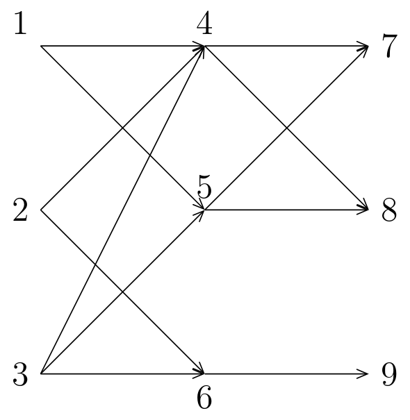
| Soit le graphe (fig. 6) dont les sommets, au nombre de neuf, sont numérotés de 1 à 9. | Let be the graph (fig. 6) whose 9 vertices are numbered from 1 to 9. |
|
|
| 1 | 4 | 5 | 6 | 7 | 9 | |
| 1 | 2 | 3 | 4 | 5 | 6 | |
| 2. Détermination des classes . Il y a six classes dont les représentants respectifs constituent la liste . | 2. Determination of the classes . There are six classes that are respectively represented by the list . |
| 1 | 2 | 3 | 4 | 6 | 7 | |
| 1 | 2 | 3 | 4 | 5 | 6 | |
| 3. Constitution des tableaux . | 3. Establishment of tables . |
| 1 | 4, 5 | ||
| 2 | 1, 2, 3 | 4, 6 | 1, 2, 3 |
| 3 | 1, 3 | 4, 5, 6 | 1, 3 |
| 4 | 2, 3 | 7 | 2, 3 |
| 5 | 4 | 9 | 4, 1, 2, 3 |
| 6 | 6 | 6, 2, 3 | |
| 4. Détermination des bons arcs:
| 4. Determining the good arcs:
|